
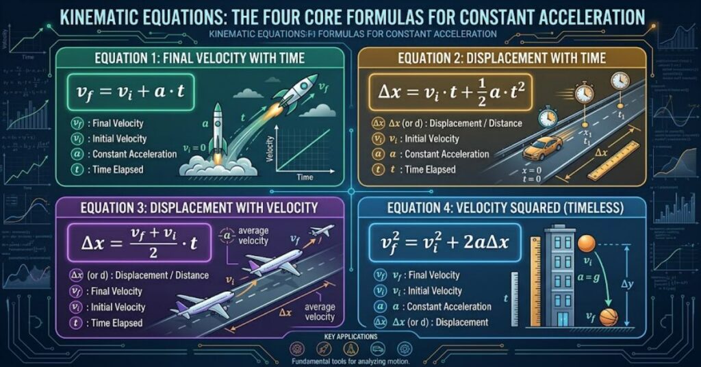
The kinematic equations are a set of core physics formulas used to describe motion when acceleration is constant. They connect displacement (Δx), initial velocity (vᵢ), final velocity (v𝒇), acceleration (a), and time (t). Rather than describing why an object moves, kinematics focuses on describing how its motion changes.
For students, these equations are among the most practical tools in introductory mechanics. They can be used to calculate how far a car travels while accelerating, how fast an object becomes after a given time, or how quickly a falling object reaches the ground.
There is one condition that should always come first: the standard constant-acceleration equations are valid only when acceleration is constant over the interval being analysed. OpenStax and Physics LibreTexts both emphasise this limitation.
A useful way to understand them is not to memorise four isolated formulas. Instead, treat the equations as different ways of connecting the same five motion variables. Once the known quantities are identified, the appropriate equation becomes much easier to select.
What Are Kinematic Equations?
In introductory physics, the constant-acceleration equations are normally presented as a group of five closely related relationships. Some teaching resources refer to four core equations because the average-velocity relationship is often treated separately. OpenStax lists the full constant-acceleration set as relationships involving average velocity, velocity, displacement, acceleration, and time.
Using Δx for displacement, the commonly used equations are:
Average velocity
vˉ=2vi+vf
Velocity after a period of constant acceleration
vf=vi+at
Displacement when time is known
Δx=vit+21at2
Velocity and displacement without time
vf2=vi2+2aΔx
The first relationship provides the average velocity needed for the displacement equation:
Δx=vˉt
Together, these relationships allow several combinations of known and unknown variables to be solved.
The Five Variables You Need to Know
Before selecting an equation, identify the variables in the problem.
| Symbol | Meaning | Common SI unit |
| Δx | Displacement | metre (m) |
| vᵢ | Initial velocity | metre per second (m/s) |
| v𝒇 | Final velocity | metre per second (m/s) |
| a | Acceleration | metre per second squared (m/s²) |
| t | Time | second (s) |
The notation can vary between textbooks. Some use v0 rather than vi, and x−x0 rather than Δx. These represent the same underlying ideas when the initial and final positions are defined consistently.
This is an important practical point: symbols may change, but the physical relationships do not.
The Four Main Equations Explained
1. Finding Final Velocity
vf=vi+at
This equation is useful when you know the initial velocity, acceleration, and time and want to calculate final velocity.
For example, suppose a bicycle begins at 4 m/s and accelerates at 2 m/s² for 5 seconds:
vf=4+(2)(5) vf=14 m/s
The equation shows a direct relationship between acceleration and the change in velocity.
2. Finding Displacement
Δx=vit+21at2
This equation is especially useful when time is known.
Suppose a vehicle starts at 10 m/s and accelerates at 3 m/s² for 4 seconds:
Δx=(10)(4)+21(3)(42) Δx=40+24 Δx=64 m
The t2 term is significant. It means displacement does not increase linearly with time when acceleration is constant. OpenStax demonstrates this distinction through position-time and acceleration relationships.
3. Finding Displacement Through Average Velocity
When acceleration is constant:
vˉ=2vi+vf
Then:
Δx=vˉt
This is particularly useful when both initial and final velocities are available.
For example, if an object moves from 5 m/s to 15 m/s over 4 seconds:
vˉ=25+15=10 m/s
Therefore:
Δx=(10)(4)=40 m
The method works because constant acceleration causes velocity to change uniformly over the interval.
4. Finding Velocity Without Time
vf2=vi2+2aΔx
This is one of the most useful equations when time is unknown or irrelevant.
Suppose an object starts at 3 m/s, accelerates at 4 m/s², and travels 10 m:
vf2=32+2(4)(10) vf2=89 vf≈9.43 m/s
The equation eliminates time completely. That makes it particularly valuable in stopping-distance and motion problems.
How to Choose the Right Equation
A common mistake is choosing an equation because it looks familiar rather than because its variables match the problem.
| Known information | Useful equation | Typical unknown |
| vᵢ, a, t | vf=vi+at | Final velocity |
| vᵢ, a, t | Δx=vit+21at2 | Displacement |
| vᵢ, v𝒇, t | Δx=2vi+vft | Displacement |
| vᵢ, v𝒇, a | vf2=vi2+2aΔx | Displacement |
| vᵢ, v𝒇, Δx | vf2=vi2+2aΔx | Acceleration |
The best workflow is simple: list the knowns, identify the unknown, then select the equation containing those quantities.
Physics LibreTexts similarly emphasises that solving kinematics problems begins with identifying the relevant quantities and choosing an appropriate relationship.
The Sign Convention Matters
Kinematic calculations become confusing when positive and negative directions are not defined.
Suppose upward is positive. In vertical motion near Earth’s surface, gravitational acceleration is approximately:
a=−9.80 m/s2
The negative sign indicates that gravity acts downward relative to the chosen coordinate system. OpenStax uses this convention for vertical motion.
A negative acceleration therefore does not automatically mean the object is slowing down. If velocity is also negative, the object may actually be speeding up in the negative direction.
This is one of the most useful conceptual checks students can make before calculating.
A Real-World Example: Stopping a Car
The equations become especially practical in braking problems.
OpenStax gives an example involving a car travelling at 30.0 m/s and compares stopping on dry and wet concrete. The cited deceleration values are 7.00 m/s² for dry concrete and 5.00 m/s² for wet concrete.
Because the final velocity is zero, the equation without time is convenient:
vf2=vi2+2aΔx
Rearranging:
Δx=2avf2−vi2
For the dry surface:
Δx=2(−7)02−302≈64.3 m
For the wet surface:
Δx=2(−5)02−302=90 m
The difference is substantial: the idealised stopping distance increases by about 25.7 m under the stated assumptions.
This example provides a useful insight beyond formula memorisation: a relatively modest change in deceleration can produce a large change in stopping distance because velocity is squared in the relevant equation.
Three Practical Insights Students Often Miss
Acceleration Does Not Have to Mean Speeding Up
Acceleration describes the rate of change of velocity. An object moving in the positive direction can have negative acceleration and slow down, while an object moving in the negative direction can have negative acceleration and speed up.
Time Is Not Always Necessary
Many beginners assume every motion problem requires time. The equation
vf2=vi2+2aΔx
shows that time can be eliminated when velocity, acceleration, and displacement provide enough information.
Constant Acceleration Can Be an Approximation
Real systems do not always maintain perfectly constant acceleration. Air resistance, changing engine force, road conditions and other factors can make acceleration vary. However, a changing-acceleration problem can sometimes be divided into intervals where constant acceleration is a reasonable approximation. Physics LibreTexts explicitly discusses this approach.
Kinematic Equations vs Dynamics
Kinematics and dynamics answer different questions.
| Kinematics | Dynamics |
| Describes motion | Explains causes of motion |
| Uses displacement, velocity, acceleration and time | Uses forces, mass and acceleration |
| Does not require knowing the cause of acceleration | Often uses Newton’s laws |
| Useful for predicting motion | Useful for determining why motion changes |
For example, kinematics can calculate how fast a car becomes after five seconds of known acceleration. Dynamics can investigate which forces produced that acceleration.
Keeping these subjects separate makes introductory mechanics much easier to organise.
The Future of Kinematic Equations in 2027
The equations themselves are unlikely to change. They are mathematical consequences of constant acceleration and remain foundational to introductory mechanics.
What is changing is how students interact with them. Digital simulations increasingly allow learners to adjust velocity, acceleration and time while observing corresponding position and velocity graphs. OpenStax, for example, connects its kinematics discussion with interactive graph-based exploration.
The more important educational shift is therefore likely to be from formula memorisation towards modelling. Students who understand assumptions, coordinate systems, units and graph behaviour will be better prepared for situations where acceleration is not constant and the standard equations cannot be applied directly.
Key Takeaways
- Constant-acceleration equations connect displacement, velocity, acceleration and time.
- The equation vf=vi+at is useful when time and acceleration are known.
- The displacement equation includes a t2 term because acceleration changes position non-linearly with time.
- The velocity-squared equation is valuable when time is unavailable.
- Negative acceleration is about direction, not automatically about slowing down.
- The equations should not be used blindly when acceleration changes significantly.
- Unit consistency and a clearly defined positive direction are essential for reliable answers.
Conclusion
Kinematic equations provide one of the clearest mathematical frameworks for describing motion under constant acceleration. Their usefulness comes from the way they connect five fundamental quantities: displacement, initial velocity, final velocity, acceleration and time.
The strongest approach is not to memorise formulas in isolation. Start by identifying what is known, define the positive direction, check the units and then select the equation that connects those quantities to the unknown. This method reduces unnecessary algebra and helps reveal whether an answer is physically sensible.
The equations also have important limits. They assume constant acceleration, so real-world situations involving rapidly changing forces may require a different model or a piecewise approach.
For students learning mechanics, that limitation is as important as the formulas themselves. Understanding when an equation applies is what turns a memorised formula into a useful physics tool.
Frequently Asked Questions
What are the kinematic equations used for?
They are used to calculate relationships between displacement, velocity, acceleration and time for motion with constant acceleration.
What are the four main kinematic equations?
The commonly taught four are vf=vi+at, Δx=vit+21at2, Δx=2vi+vft, and vf2=vi2+2aΔx. Some textbooks present the average-velocity relationship separately.
When can kinematic equations be used?
The standard equations apply when acceleration is constant over the interval being analysed.
Which kinematic equation does not use time?
The equation vf2=vi2+2aΔx does not contain time, making it useful when time is unknown.
What is the difference between velocity and acceleration?
Velocity describes how position changes with time, while acceleration describes how velocity changes with time. Acceleration can be positive or negative depending on the chosen coordinate direction.
What value is used for gravitational acceleration?
Near Earth’s surface, gravitational acceleration is commonly approximated as 9.80 m/s2. Its sign depends on the coordinate system selected for the problem.
Do kinematic equations work for projectile motion?
They can be applied to each component of projectile motion when the relevant acceleration is constant. Near Earth’s surface, horizontal acceleration is commonly taken as zero while vertical acceleration is approximately −9.80 m/s2 when upward is defined as positive.
Methodology
This article was researched using current educational physics sources, primarily OpenStax and Physics LibreTexts. Their explanations were used to verify the constant-acceleration assumption, equation forms, variable definitions, gravitational acceleration and problem-solving principles.
The numerical braking example is independently calculated from the values presented in OpenStax’s constant-acceleration example. The article does not claim firsthand laboratory testing, interviews or original experiments. Named educational examples are used as documented case material rather than presented as personal observation.
A key limitation is that the standard equations describe an idealised constant-acceleration model. Real motion can involve changing acceleration, air resistance, friction and other effects. The equations should therefore be treated as a model whose assumptions must be checked before application.
References
OpenStax. (2020). Physics: 3.2 Representing acceleration with equations and graphs. Rice University.
OpenStax. (2020). Physics: Ch. 3 key equations. Rice University.
OpenStax. (2022). College Physics 2e: 2.5 Motion equations for constant acceleration in one dimension. Rice University.
OpenStax. (2017). University Physics Volume 1: 3.4 Motion with constant acceleration. Rice University.
LibreTexts. (2022). One-dimensional motion: The constant acceleration equations. Physics LibreTexts.
Park, A. (2024). Kinematics. Physics LibreTexts.